Color Science From the Purview of H.265

A few months ago I was given the task to integrate a Vulkan video encoder into our renderer, which would compress frames in H.264/H.265. I went in knowing nearly nothing about video compression and came out with some interesting knowledge I will cover in this new series. This article goes over color-related topics such as chroma subsampling, color gamuts, color spaces and some color science math.

---

When compressing video into H.265, a whole gang of parameters can be set to customize the compressed video stream. If you are unfamiliar with video compression concepts, a lot of these parameter names probably sound alien. Here are just a few:

• colour_primaries
• transfer_characteristics
• matrix_coeffs
• chroma_format_idc
• pic_width_in_luma_samples

While having to cross-examine and iterate over all these parameters, I was introduced to interesting concepts related to video compression, some of which I will cover today. The following article includes deep and shallow dives into concepts related mostly to color.

If you are interested in my adventure with compressing H.264/H.265 using Vulkan Video, check out some of my previous articles: H.264 Vulkan Video Encoding, H.265 Vulkan Video Encoding, and Debugging Strategies. Otherwise, let's dive into COLOR!

Color spaces and color gamuts, the opening of a rabbithole: what is color, anyway?

note

Related H.265 parameters (VUI): colour_primaries, transfer_characteristics, matrix_coeffs

colour_primaries is a VUI parameter which indicates what color space the source video was in. For example, if set to 1, this indicates the source video is in the Rec. 709 color space, which is the standard RGB color space. In Rec. 709 color space, [255,0,0] corresponds to red.

// This indicates our source video is in Rec. 709 color space.
vui.colour_primaries = 1;
vui.transfer_characteristics = 1;
vui.matrix_coeffs = 1;

However H.265 video is always encoded in YUV color space, which uses Y’CbCr instead of RGB. In this space, red would be something like [54, 99, 255]. There’s always a conversion from source color space → YUV color space that must happen before encoding.

VUI parameters are essentially metadata for decoders and display systems. colour_primaries is used by decoders to know what color space the decoded YUV color data should be converted back to after decoding it.

I had an idea about what RGB color coordinates were, but…what about Y’CbCr coordinates? What is the difference between YUV and Rec. 709 color spaces, and why is H.265 encoded in YUV? But my main question was: what is a color space really?

Oh but all this opens a much bigger question: what is color? It is tempting to free fall into this rabbithole.

Light and color

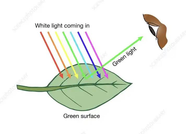
The sun emits electromagnetic radiation of different wavelengths but that travel at the same speed (the speed of light, 3 million m/s). Some of this light is visible to us, and so we call this the visible spectrum, and all light outside the visible spectrum appears to us as black (e.g. uv light). All frequencies that comprise the visible spectrum are present in roughly equal quantities in a sample of sunlight. This is our unadulterated white light. Thank you, sun.

"The mooooon, beautiful. The sun, even more beautiful." - Oh Yeah, by Yello

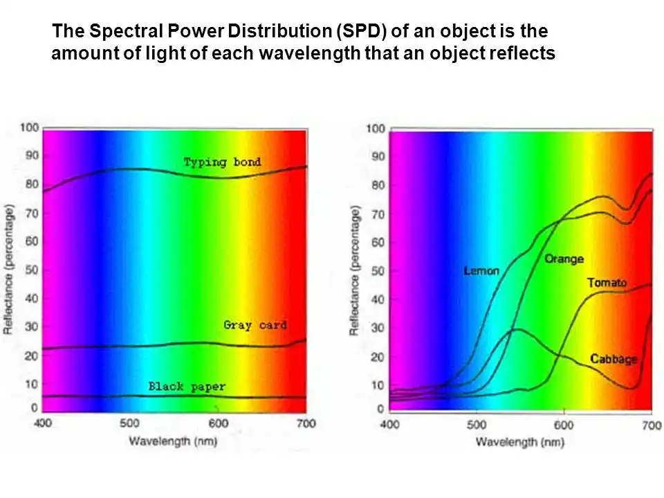
Then, light hits materials, and some of the light is absorbed and some of it is reflected. A green leaf reflects green light and absorbs all of the rest. This interaction with materials creates an imbalance in the light’s spectral power distribution which is a fancy term to describe the relative proportion of different frequencies that are present in a given sample of light. This is how our white light is chopped and screwed by the environment.

Green light is reflected by a leaf. In fact there is also some light that comes out the other side of the leaf (not shown in the diagram above). This is called transmitted light. In dense forest canopies, plants lower on the ground have adapted to utilize this filtered light for photosynthesis.

The spectral power distribution describes how the power of a light source is distributed across different wavelengths of the electromagnetic spectrum.

Color is simply a sensation that is produced in our minds after our eyes take in light. Color is a subjective sensation, not a property of the physical world. It is an engaging hallucination that we have been gifted with, complementary of consciousness. More pragmatically, it is a useful evolutionary trait we’ve developed to discern different materials in our environment. Color pops out.

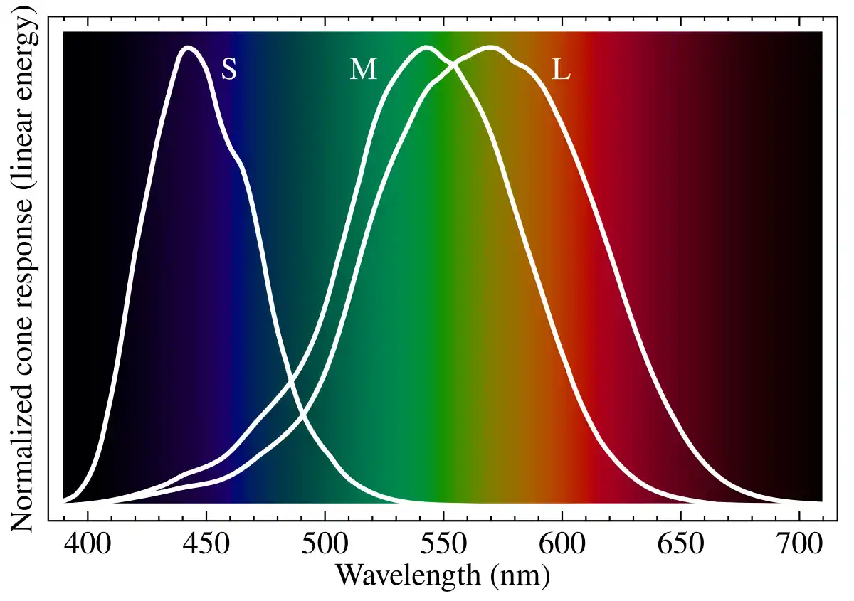
Inside our eyes there are three different types of cone cells, which react to different ranges of the visible spectrum. Let’s call these different cone cells L, M, and S for long, medium and short wavelengths. L response peaks at 575 nm, M peaks at 535 nm, and S peaks at 445 nm. This is why they are sometimes referred to as the red, green and blue cone cells, although they each react to a wide range of colors. Here is how each cone responds to different wavelengths of light:

Every wavelength of light activates a response in at least two different types of cones.

The back of our eye is lined with a thin layer called the retina. The retina is composed of photoreceptors. There are two types: cone cells (which react to color) and rod cells (which react to very low levels of light, but in grayscale).

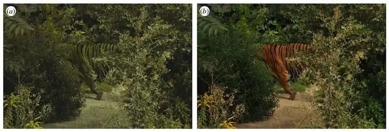
Humans have trichromatic vision. We have three independent channels for conveying color vision which respond to variations of red, green and blue. However, many terrestrial mammals, including dogs, cats, horses and deer, have dichromatic vision, possessing only two cone cells. Consider a dog - possessing only blue and yellow cone cells - peering at a rainbow. A human sees an arched array of red, orange, yellow, green, blue, violet but a dog simply sees a spectra of blues and yellows. Reds and oranges are missing in most dichromatic mammalian vision. This is what makes tigers excellent at camouflage for their desired audience, e.g. deer and boars.

(a) Dichromatic vision. This is what the tiger’s prey sees, and also what colorblind humans see, since they only possess green and blue cone cells. (b) Trichromatic vision. This is what humans see.

Different spectral power distributions (combinations of light) can result in the same L, M and S values which are sent to the brain. For example, a yellow light results in the same LMS values as the combination of a red and green light. This phenomenon is called metamerism.

We need a system to recreate the spectral power distribution that will result in a certain color inside the user’s brain. This is a color space. A color space is a mathematical representation of a certain finite range of colors. It is a system for recreating different color sensations. We call the finite range a color space can describe a color gamut.

CIE XYZ color space, or the Visible Human Color Gamut

CIE stands for la Commission Internationale de l’Eclairage, established in 1913. You may consider the CIE to be the scientific authority on light. The most famous color space is the CIE XYZ color space, developed in 1931, which describes the visible human color gamut. Maybe you’ve seen this horseshoe-shaped diagram before, referred to as the chromaticity diagram. This is actually a 2d cross section of a 3d shape. The 2d part below, i.e. the x and y axes, specify the color (chroma) and the z axis specifies the brightness (luminance). The closer z gets to 0 the less bright the color at that [x, y] point is. It is often shown in 2d for simplicity.

CIE 1931 xy chromaticity diagram. These are the colors at their most saturated (with highest luminance).

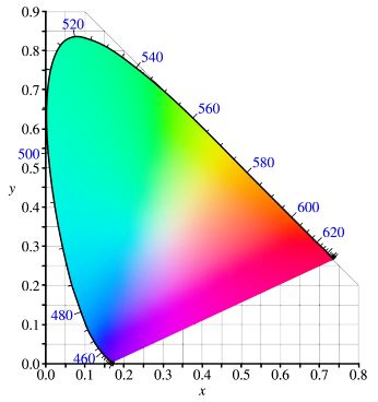
What is special about the CIE 1931 xy chromaticity diagram is that if you take any two points and draw a line between them, all the colors on that line will be proportional variations of the two colors at the endpoints. If you read the deep dive below, the reason for this is explained.

Deep dive into the math: how did we plot all visible human colors into a 3d shape?

🚨 This is a deep dive. Feel free to skip to the next section if you feel indifferent about the explanation behind this, or want to keep it moving. You don’t need this to understand the rest of the article.

After finding the chromaticity diagram I felt angry because I did not understand. How was this diagram even come up with? How is it possible to know the visible human color gamut? Isn’t color a subjective experience? How can we possibly measure and plot it?

Finding the answer to this question frustrated me to no end until I came across this excellent video by Kuvina Saydaki, which explained it all:

The Amazing Math behind Colors!

I’ll resume some key points from his video. Let’s start with out first “axiom”. We know the cone responsivity spectra:

Normalized cone responsivity spectra.

How do we know this? Earliest attempts to measure cone sensitivity date from the 19th century. Arthur König and Conrad Dieterici published a paper in 1886 entitled "Fundamental sensations and their sensitivity in the spectrum", but if you are really curious as to how they did it, do your own research.

The range of colors that we see are all the possible combinations of L, M and S. Let’s construct a normalized LMS space with L, M and S corresponding to x, y and z axes respectively. Now this should mean that the range of possible colors should cover a cube of dimensions [1,1,1].

However, there are certain possible combinations of [l, m, s] that are impossible. Consider l=1, m=0, s=0. Take a look at the normalized cone responsivity spectra. There is no possible combination of wavelengths that could result in those values, mainly because the L and M response curves overlap over the same wavelengths.

Fun fact, science alert: we call the “color” that could be described by such an impossible combination an impossible color. Our brain can simply never receive that combination (and even if it did, how would it react? Would a new color be displayed?). If we take a look back at the CIE chromaticity diagram, all the white space that is around the horseshoe are “impossible colors”. Keep in mind that we are working our way up to translating this LMS space into this CIE XYZ space.

The color at the coordinate [0.5, 0] is an impossible color. Imagine?

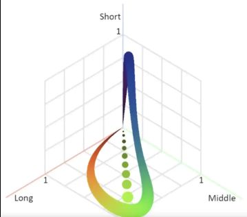
1. Plot the spectral colors

The next step is to plot the three cone response curves onto our LMS space. We have the L, M and S axes which correspond to x, y and z. However we can’t really define a function whose output (z-value) can be defined as:

🎨

$z = f(x, y)$

The L, M and S values are not dependent on one another. Rather they are functions of another variable entirely: the wavelength. Therefore we can use parametric equations to define our x, y, z:

🎨

$x=L(t)$

$y = M(t)$

$z = S(t)$

where $t$ is the wavelength λ, and $L$, $M$ and $S$ are the response curves

We get something like this:

Normalized cone responsivity spectra.

Normalized cone responsivity spectra plotted into LMS space, using the parametric equations shown above.

This allows us to get the exact L, M and S values for one specific wavelength of light λ. Therefore we have a graph which works for monochromatic light (light which contains photons of one certain wavelength).

2. Plot luminance

We can also plot the luminance (or, brightness) of a particular light. Luminance in fact corresponds to the amount of physical light photons received per area of a sample of light. Take a green light (520 nm), which gives the approximate LMS values:

$L = 0.63, M = 0.82, S = 0.029$

When a less bright green light enters your retina, the L, M and S cones will still be hit, but only a smaller proportion of them. The signal sent to your brain is then just a smaller proportion of the green LMS value. So a color and all of its variances in luminance can be described as:

🎨

$luma * [l, m, s]$

where luminance $luma$ goes from 0 to 1, and $l,m,s$ are the values of the color at highest luminance

In our LMS space, this corresponds to the vector that goes from $[0, 0, 0]$ to the color $[l, m, s]$. You can visualize it below for the color green:

3. Plot the combinations of spectral colors

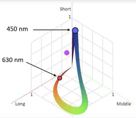
Now think back to the spectral power distributions of different materials. Most colors we see in nature are in fact a mixture of light of different wavelengths. This is called polychromatic light. A mix of blue and red light creates the color magenta in our brain. How does magenta fit into our LMS space?

When the eye receives a combination of photons of different wavelength, the eye will compute l, m, and s values proportionally to the wavelengths received. Say it received an equal portion of red ($λ_{1}$) and blue ($λ_{2}$) light. Then half of the cone cells receive the red light and half receive the blue light. We get:

🎨

$l = 0.5 * L(λ_{1}) + 0.5 * L(λ_{2})$

$m = 0.5 * M(λ_{1}) + 0.5 * M(λ_{2})$

$s = 0.5 * S(λ_{1}) + 0.5 * S(λ_{2})$

where $λ_{1}$ is red light wavelength, $λ_{2}$ is blue light wavelength, and $L$, $M$ and $S$ are the response curves

In the LMS space magenta is the midpoint of the line connecting the blue color point and red color point. $c_{magenta} = 0.5 * c_{blue} + 0.5 * c_{red}$.

Magenta is the weighted average of the blue and the red point.

The varying proportions of light at different wavelengths received by the eye will translate to the varying proportions of LMS values of those different wavelengths. The LMS signals are added and sent to the brain.

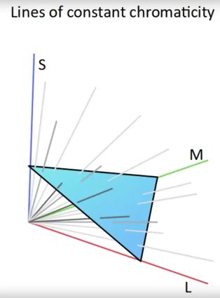
Therefore we can see that the set of possible values in LMS space is the weighted combination of all spectral colors. Mathematically, we describe this as a convex combination of all spectral colors.

🎨

For the points $c_{1}, c_{2}, ..., c_{n}$ found on the $L$, $M$ and $S$ spectral curves, the set of points described by:

$α_{1}c_{1} + α_{2}c_{2} + ... + α_{n}c_{n}$ where $α_{i}\geq0$ and $α_{1} + α_{2} + ... + α_{n} = 1$

corresponds to all the visible colors.

Geometrically, this is the convex set contained by the L, M and S curves. This is how we get our 3d shape. This is called the visible gamut, and any color you can think of is somewhere within it! Everything outside of it but still within our LMS cube are the invisible colors.

This is the convex set of visible colors…already looking closer to the horseshoe.

The last step is to make our 3d visible color gamut form a 2d chromaticity diagram. As discussed before all lines going from the origin to any point have the same chromaticity but varying luminance. What we need is a 2d cross section of our 3d shape at a certain given luminance, to have a view of all chromaticities!

This is in fact how CIE developped the famous “horseshoe” chromaticity diagram. However rather than directly using the LMS space, it used the CIE 1931 xyz space, which is a linear transformation of the LMS space (every point multiplied by a matrix!) which helps account the non-normalized responsivity spectra. Note that to construct our LMS space we’ve been using the normalized LMS curves, but in reality, the curves are something more like this:

The CIE 1931 xyz space transforms each point in LMS space by a specific matrix to account for this variance. It looks similar to LMS as you can see below.

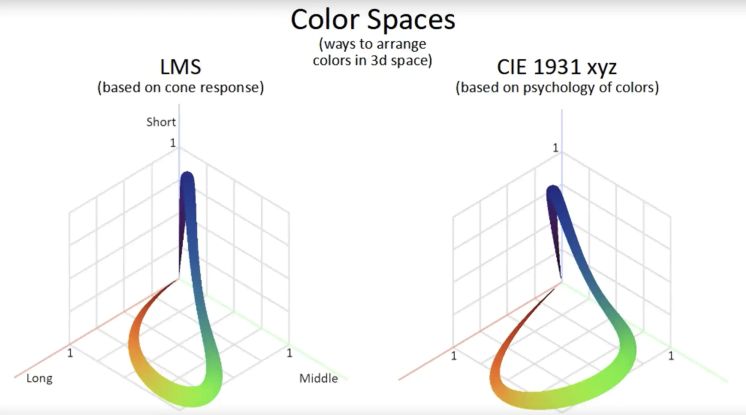
If we take a 2d cross section of the CIE 1931 xyz space we finally get our chromaticity diagram! Woo!

Color gamuts within color gamuts

So now, I am finally making my way around to the answer of my original question: what is the Rec. 709 color space which I have assigned to my VUI parameter colour_primaries?

The Rec. 709 color space is defined by the combination of three color primaries (red, green, blue) which are at [0.64, 0.33], [0.3, 0.6], and [0.15, 0.06] on the CIE 1931 xy chromaticity diagram. All of the colors contained within the area of the triangle are part of Rec. 709 color gamut. Setting colour_primaries to 1 informs that the color primaries above are used for RGB color data.

Another well known color space is Rec. 2020 which has its red, green, blue color primaries at [0.708, 0.292], [0.17, 0.797] and [0.131, 0.046] in the xy chromaticity diagram. Rec. 2020 describes a wider color gamut than Rec. 709, and in fact encompasses the Rec. 709 color gamut.

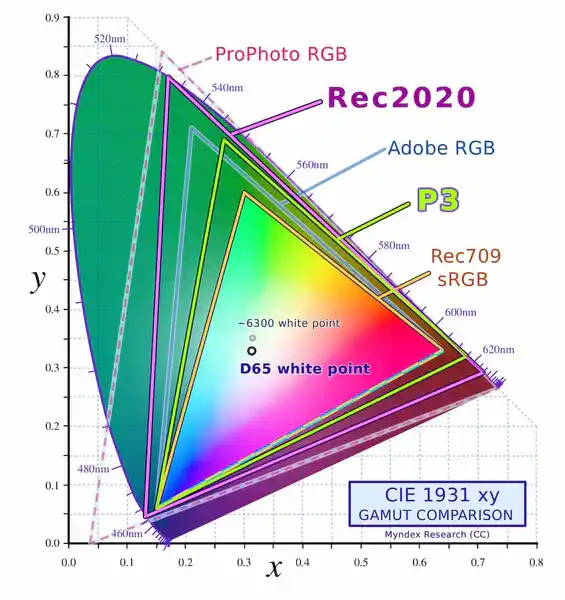
The CIE 1931 is what is known as an absolute color space. Rec. 2020 and Rec. 709 are relative color spaces. A color coordinate described in those spaces are relative to their color primaries. (1,0,0) in Rec. 709 corresponds to xy = [0.64, 0.33] whereas (1,0,0) in Rec. 2020 corresponds to xy = [0.708, 0.292].

To convert between relative color spaces, first a conversion from source color space to absolute color space is made, and then from the absolute to destination color space.

YUV color space

YUV color space, unlike RGB type color spaces, separates image information into luminance and chrominance components.

YUV Components:

• Y (Luma): Brightness/luminance information - represents how light or dark each pixel is
• U (Cb): Blue-difference chroma - represents the blue-minus-luma (B-Y) color difference signal
  • positive Cb: the pixel has more blue than the average luminance would suggest
  • negative Cb: the pixel has less blue (more yellow/orange)
• V (Cr): Red-difference chroma -represents the red-minus-luma (R-Y) color difference signal
  • positive Cr: the pixel has more red than expected
  • negative Cr: the pixel has less red (more cyan/green)

Example of U-V color plane, Y′ value = 0.5, represented within RGB color gamut

Any color gamut (with any color primaries) can be converted into YUV color space. Separating luminance from color makes compression more efficient (see chroma subsampling). This is why all H.264/H.265 converts video into YUV color space before encoding.

A relevant musical interlude

I listen to a lot of ambient music while I research and code. Brian Eno is always entering and exiting my brain. He made an album with his brother Roger called Mixing Colours that is relevant to certain topics discussed. Within it are spatial meditative pieces inspired by colors: Deep Saffron, Obsidian, Cerulean Blue, Dark Sienna, Wintergreen, Burnt Umber, etc. If you are new to ambient music, I recommend it as something to listen to while doing something else. Do not expect yourself to be entertained by it. Treat it as an accompaniment to your thoughts, and other daily activities, as you would the rays of sunlight intermittently siphoned off by clouds. The music is meant to hollow out your brain to conjure concentration, or conscious presence.

Brian and Roger Eno - Mixing Colours

An ambient album with songs that imagine mixed colors

Chroma subsampling

note

Related H.265 parameters (SPS): chroma_format_idc, pic_width_in_luma_samples, pic_height_in_luma_samples

chroma_format_idc is a SPS parameter which specifies whether the video should be compressed using chroma subsampling, and what level of chroma subsampling.

// This indicates we want to encode in chroma format 4:2:0.
// Other options: 4:2:2, 4:4:4.
sps.chroma_format_idc = STD_VIDEO_H265_CHROMA_FORMAT_IDC_420;

Chroma subsampling is a compression technique that reduces color data (chrominance) while preserving brightness (luminance) data. H.264/H.265 are not encoded in RGBA format but in Y’CbCr (a.k.a. YUV) color space which encodes color in chroma and luma.

It turns out human vision is most reliant on the varying luminance (rather than chrominance) of an image to make out the detail of it. Think of the crispness of a black and white image. Although a black and white image lacks the warm information of color, there is nothing lacking in its detail.

It turns out if the image is lacking chroma data it is more difficult for to us to notice a decrease in quality in comparison to if it lacked luma data. So the idea behind chroma subsampling is to shave off chroma data of some pixels while preserving all luma data of pixels.

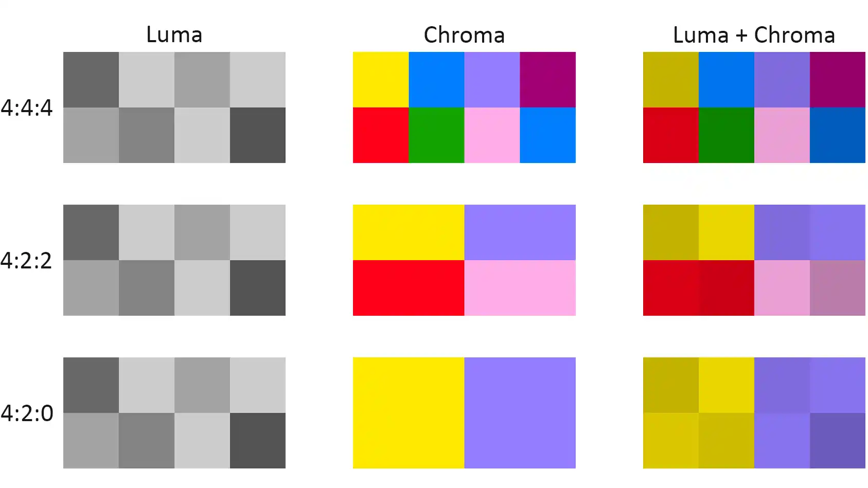
In a 4:4:4 video, no chroma is removed (no compression).

In a 4:2:2 video, every other chroma pixel is removed in the same row.

In a 4:2:0 video, every other chroma pixel is removed in the same row, AND every other chroma pixel is removed in the same column.

By now you must understand why the variables for frame width and height are pic_width_in_luma_samples and pic_height_in_luma_samples . Luma is never compressed so the number of luma samples is equal to the number of pixels.