Rendering 3dverse

Vulkan delivers exceptional performance at the cost of verbose code and meticulous resource management, making even basic rendering operations unnecessarily complex. All this verbosity kills rapid experimentation and makes simple tasks tedious.
At 3dverse, we built a visual render graph system on top of Vulkan that replaces hundreds of lines of boilerplate with connected nodes that automatically handle the low-level details.
In this post, I'll demonstrate our approach with a simple screen-clearing example, reveal the production PBR render graph powering our cloud rendering platform, and finally if you are still around, preview our new ray tracing capabilities.

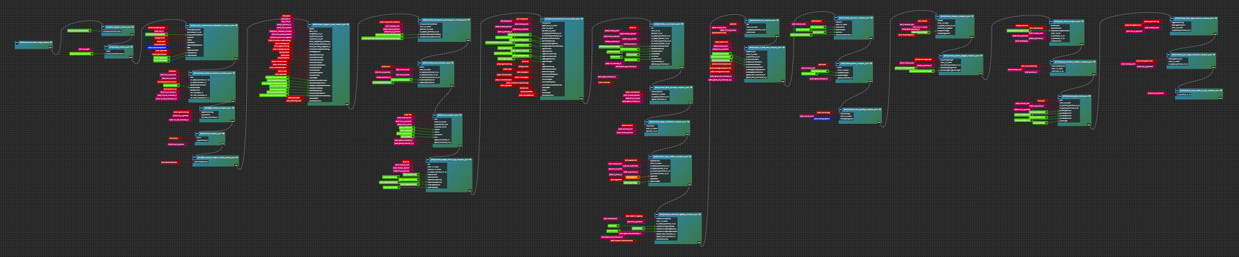
That complex-looking diagram up there is our Default PBR render graph at 3dverse - the visual representation of our rendering pipeline. It represents years of our team's work to simplify Vulkan development and avoid drowning in its boilerplate.
And hello wonderful person! I've been the resident rendering mystic at 3dverse for about five years now. Creating the system that powers the render graph above involved debugging colorful issues, studying specifications and research papers, and, naturally, drinking plenty of coffee.
At 3dverse, we created a thin visual abstraction layer over Vulkan that we use to create sophisticated rendering pipelines without having to write raw Vulkan code! It powers the rendering in our cloud native platform, where a server in the cloud does the heavy lifting by rendering an image that is then streamed.
Over the next few posts, I want to share a slice of what we've created after all this time. Not the struggle to build it, but the elegant system that emerged from years of iteration.
A Simple Example That Doesn't Do Justice To Years of Work
Let me demonstrate how a task that requires writing an excessive number of lines of C++ Vulkan code can be made visually in seconds. And that task is clearing the screen to a color.
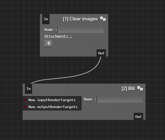
In order to display anything on the screen in 3dverse we will need to first create a render graph. A render graph is an asset in 3dverse that is basically a connected graph that tells the GPU what operations to perform and in what order.
Each node in this graph encapsulates Vulkan operations that would normally require more than one line of setup code, proper synchronization, and resource management. The connections between nodes represent how data flows through the rendering pipeline.
The Minimal Render Graph
The simplest functional render graph we can create just clears the screen to a color:
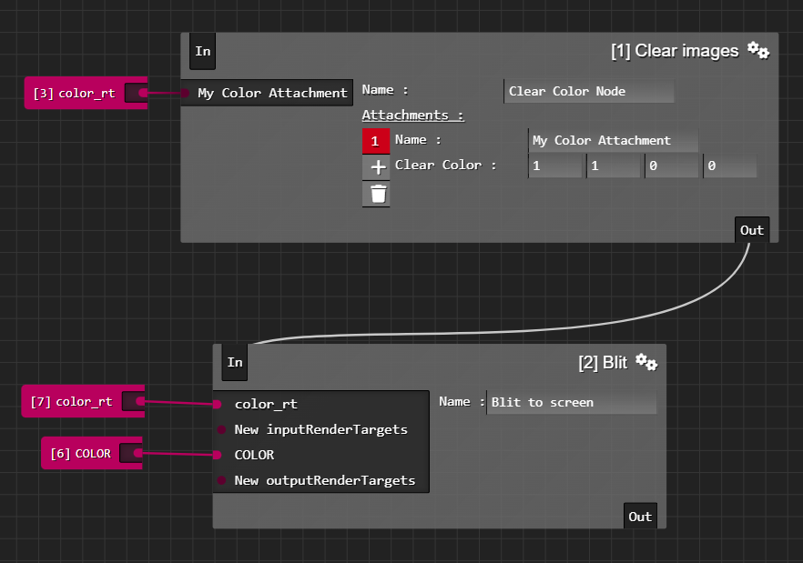
What we are seeing is deceptively simple. Underneath these two nodes lies an entangled but orderly mess of tightly crafted code. We need two nodes to make this work:
- A Clear Images node (which fills our texture with a color)
- A Blit node (which will copy our texture to a destination for display on screen)
These two nodes provide some services, and their clients are render targets. Render targets are texture resources in 3dverse that serve as destinations for rendering operations.
Render targets are created in their own tab in the editor. And once we create them, we can drag them onto the render graph, and then connect them to graph nodes.
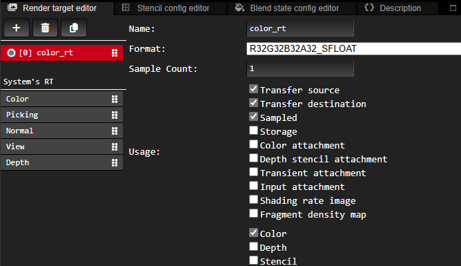
Now we connect the nodes and assign render targets to node inputs: the Clear node receives our render target as input with its clear color set to yellow, while the Blit node takes this cleared render target as input and outputs to the system's "Color" render target, which is displayed on screen when the frame completes.
When you press build, our compiler transforms this visual graph into a proper Vulkan execution chain - handling descriptor sets, image transitions, synchronization primitives, and all the verbosity that makes Vulkan fun.
The final step is simply assigning the render graph to the main Camera. The Camera is an entity with a Camera Component attached that is created automatically for each user.

Our scene structure is built around entities (basic scene objects) that hold various components. The camera component is particularly important for rendering, as it determines what view of the scene gets rendered using our graph.
And after all this, we see yellow! Magnificent.

This yellow represents years of work making the difficult appear effortless. But as a pro tip: if you only need to display a yellow color on the screen, a simpler approach could be to use MS Paint and its Fill feature.
From Minimal to Production: Our Main PBR Render Graph
While the yellow screen example was compelling and showed the basics, here's what our real production rendering pipeline looks like:
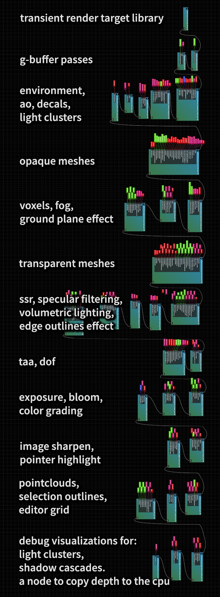
The Default PBR Render Graph shown above is our engine's main rendering pipeline.
Each node in this graph represents a subsystem that evolved through multiple iterations, and they are graphs themselves. And so graphs contain a hierarchy of more graphs, that are each connected to nodes and more graphs and render targets, and reconnected many times.
So many dots were connected in the making of these render graphs.
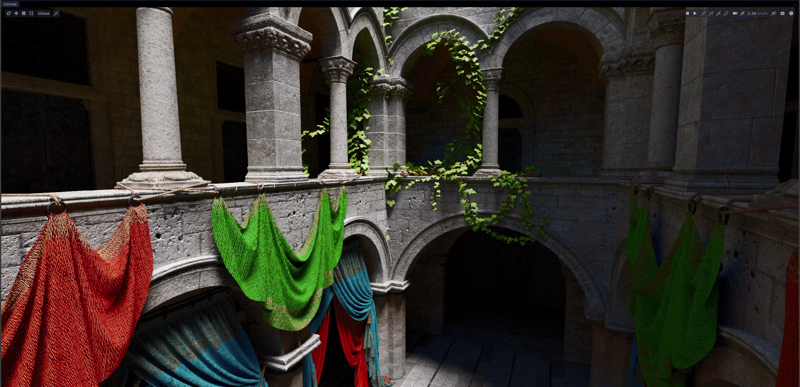
Ray Tracing Render Graph
Our latest addition is ray tracing support! Despite the verbose technology underneath, the graph still remains elegantly simple. The beautiful output below comes from a graph that's almost as simple as our yellow screen example, with just one node for dispatching the ray tracer, that is enhanced by color grading and other effect nodes.
What's Next
In the upcoming posts, I'll demonstrate our compute shader integration. Compute shaders enable more elegant effects, such as more sophisticated color clearing operations.
I will also dive into how our shader graph system lets us create custom materials for rendering geometry without writing GLSL code directly.